This article will walk through how I wrote a piece of software called ByteBass. I had the great fortune of being able to work with two of my closest friends (Neville and Sanat) and I had alot of fun working on it with them. This project was challenging and also required extensive knowledge outside of our curriculum to execute, but it’s probably my favourite school project to date.

I will try my best abstract away or at least simplify complex concepts we had to deal such as fast fourier transforms, finite state machines, fundemental frequencies, audio compression and much more. I aim to give a high level overview of the project as a whole, so I wont delve into the code much, but if you are interested in full technical specifics, you can take a look at our full project report and our project repo!

Oh also it’s also written entirely in C. Which I think is kinda cool.

What does ByteBass do?

ByteBass is a piece of software that allows bass players to identify what notes they played.

Its actually more than that, it takes a WAV file and a CLI input of what scale you played, and then it identifies what notes you played wrongly, but let’s stick with this definition for simplicity’s sake.

Plan of Attack

This project is pretty complicated, so I’ll simplify it into 3 distinct parts:

We are essentially looking at the binary contents of an audio file (literally the 1s and 0s) and trying extra geometric data.

Then from the geometric data, we can then infer what note is being played.

I promise you it’ll make more sense as we go along so hang in there.

1. Sound and its Properties

The following chapter is going to be a quick introduction to some of the physics of sound waves and how they relate to our project, so bear with me here. Its gonna focus on the second half the above flowchart, inferring what note has been played from the geometric graph.

We did some (really extensive) digging and research, and I’m going to try and distil it down to the ones most relevant to this project:

1.1 Modelling sound as a geometric wave

What is sound? It’s nothing more than vibrating air. Your mom shouting, a cricket chirping, your favourite Taylor Swift song, its all just different variations of vibrating particles. Here’s a gif to explain:

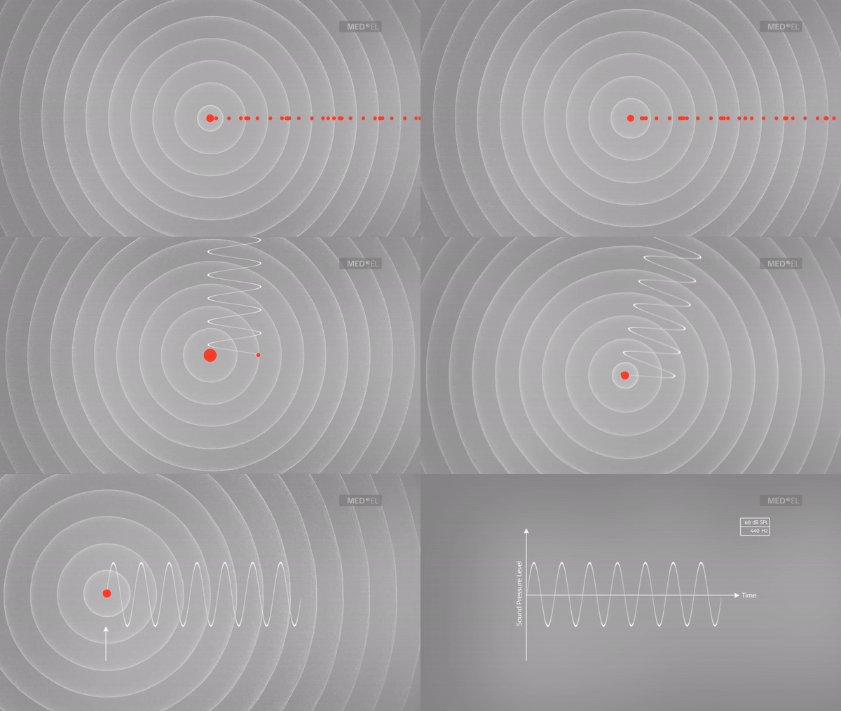
Understanding this visualisation is key! Notice how we can model the lateral, back and forth movement of the sound particle using a graph, specifically a geometric wave function.

1.2 Inferring a note from a geometric wave

But what makes a C note, a C note? A sound wave has many different characteristics, but the key property that determines how does a note sound is the frequency of the wave itself, so lets just focus on that.

Heres an audio snippet of a C note I generated using code:

It sounds pretty bland doesnt it.

It’s graphical representation is also very simple, it’s characterised by a simple sine wave of frequency around 262 Hz (the particles vibrate at a frequency of 262 times a second). Look at how nicely shaped it is.

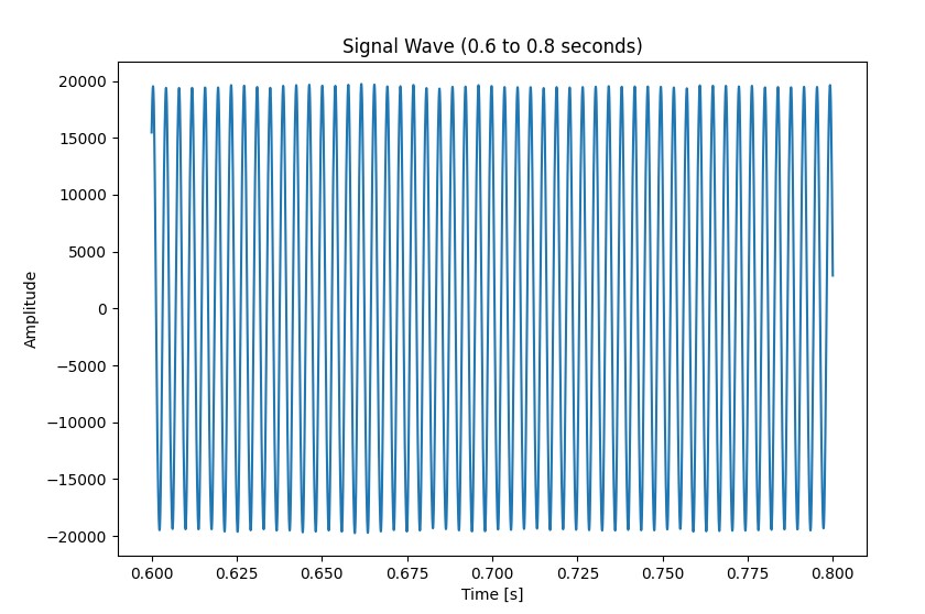
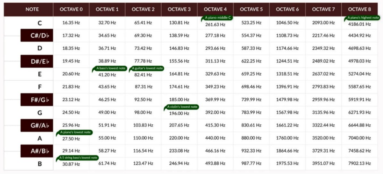
Each note in music theory has a specific frequency associated with it, since the soundwave is pretty simple, we can quickly calculate the frequency. We can then cross-reference the frequency to a chart such as the one below to find out the note being played.

1.3 Imperfections of soundwaves

Let’s take a look at that piece of audio and its corresponding graph again.

It looks really perfect and clean right?

In reality, sound waves are rarely flawless, their graphical representations are often messy and imperfect. Here’s an audio snippet of another note, but played on a saxophone:

How does that sound compare to the earlier snippet? Warmer? More human maybe? Here’s its graphical representation:

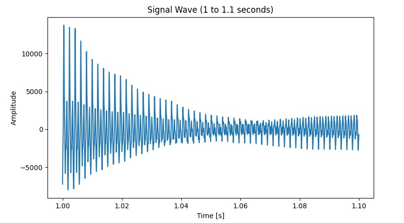
Damn this does not look as clean as the previous graph. In reality, particles rarely follow a fixed frequency, and often move in an irregular manner.

1.4 Fundemental Frequency using Fourier Transform

So does the waveform above still have a frequency?

The answer is yes, no matter the wave form, we can still extract a fundemental (or a number of fundemental frequencies)

The messy wave form above is actually a combination of many frequencies, but it still has a fundemental frequency of 1040Hz (C6).

Okay so we know now, even with messed up waveforms, we still can extract the fundemental frequency to determine what it sounds like.

But how do perform this extraction? We were pointed towards a mathematical transformation called the Fourier Transform. It’s not exactly the simplest concept to understand, so I’m outsourcing the explaination to this youtube video:

If you dont have the patience for this, THATS FINE. I get it. We all use Tiktok, we can’t do 20 minute videos anymore. We can black box this entire concept and move on.

Just remember the tldr: We can extract the fundamental frequency of any soundwave using Fourier transformations, and we can infer the perceived note from that fundamental frequency.

1.5 Summary

We’ve come to end of this section, if you’ve been only skimming, here’s a quick summary of what we’ve covered this chapter

Given the geometric data of a soundwave (sinusoidal wave), we can infer the note that’s being played by calculating the frequency of that wave, and then cross referring that to a frequency chart to find out the corresponding note.

2. Audio Data: WAV files

Okay now we know how to obtain information if we are given sound data in the geometric wave form. We should be able to extract the note that’s being played given this geometric data. Hence, we will be focusing on the first half of the flowchart for this section:

The question is now how can we extract this geometric data from the binary data within the an audio file (specifically, a WAV file) ?

Let’s take a deep dive into an audio file (WAV file) and what it contains. This is what it looks like at its lowest level.

1010101101011001110010110111010100100101111001010111001010101110111001010101010011010101100111001100101110111011010101010010101101011001110010110111010100100101111001010111001010101110101010110101100111001011011101010010010111100101011100101010111011100101010101001101010110011100110010111011101101010101001010110101100111001011011101010010010111100101011100101010111010101011010110011100101101110101001001011110010101110010101011101110010101010100110101011001110011001011101110110101010100101011010110011100101101110101001001011110010101110010101011101010101101011001110010110111010100100101111001010111001010101110111001010101010011010101100111001100101110111011010101010010101101011001110010110111

What the hell are we looking at? Looks absolutely meaningless doesnt it? But there is a method to the madness. Hidden in this binary is actually all the information we need to construct the geometric wave form that represents sound.

If you are not familiar with binary (and its ability to represent information like numbers, letters and symbols), it might be helpful looking at this video:

We’ll be splitting this massive chunk of binary into two parts: Headers and Audio Data

2.1 Header and Metadata

The first section of an uncompressed WAV file is pretty standard, it’s going to be exactly 44 bytes long, and it contains use essential data such as bit rate, sample rate and the size of the file.

Here’s a sneak preview of sample struct of the header in C:

struct wav_header
{
  char riff[4];           /* "RIFF"                                  */
  int32_t flength;        /* file length in bytes                    */
  char wave[4];           /* "WAVE"                                  */
  char fmt[4];            /* "fmt "                                  */
  int32_t chunk_size;     /* size of FMT chunk in bytes (usually 16) */
  int16_t format_tag;     /* 1=PCM, 257=Mu-Law, 258=A-Law, 259=ADPCM */
  int16_t num_chans;      /* 1=mono, 2=stereo                        */
  int32_t srate;          /* Sampling rate in samples per second     */
  int32_t bytes_per_sec;  /* bytes per second = srate*bytes_per_samp */
  int16_t bytes_per_samp; /* 2=16-bit mono, 4=16-bit stereo          */
  int16_t bits_per_samp;  /* Number of bits per sample               */
  char data[4];           /* "data"                                  */
  int32_t dlength;        /* data length in bytes (filelength - 44)  */
};

Dont worry if it all seems like gibberish, most of it isn’t really relevant to understanding our project. Just know that a good chunk of binary at the start this file is reserved for this data.

2.2 Audio Data

This is the bulk of the WAV file, where we can find the audio data itself.

Unfortunately, it’s still a massive mess of 1s and 0s, but embedded in it is actually the data we need to construct a geometric wave.

We read the binary in sets of 8 bytes (64 bits), with each set of 8 bytes representing a float (a decimal number).

What does this decimal represent? It actually represents the distance between a discrete point on the curve to the X-axis itself on the geometric wave! Here’s a photo for visualisation:

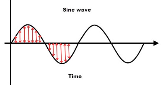
I hope this is beginning to make sense, as you can see we can read each float and construct a geometric function consisting of individual discrete points.

The smaller the gap between the floats (the greater the number of floats per unit time), the greater the fidelity of the geometric wave.

So this is how we construct the geometric wave from binary data!

3. Data slicing

We are almost there! We now know how to extract a geometric representation of a sound wave from the binary data of an audio file, and then infer the note from the sound wave itself.

We still have a problem though. The previous examples all assumes that the audio file only contains a singular note, what if multiple notes are played within the file itself?

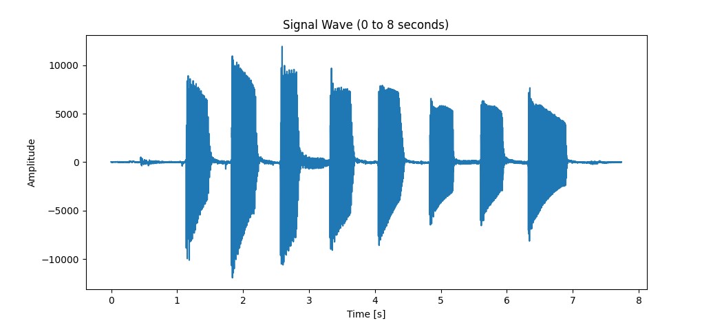
We clearly need to slice this data up for processing, but how do we do this programmatically? It seems straight forward, intuitively we can just set a hard limit on the amplitude right? If the soundwave goes past a set amplitude, we’ll just mark it as the beginning of a new note, and if it drops below it, then the note has stopped playing.

Unfortunately, we can’t do that. Different audio files have different properties that would interfere with this method. An audio file where you play the bass softly would not trigger the detection, or a bass file with high background noise would trigger the threshold but not deactivate it.

We found an elegant solution in the form of a moving average detection algorithm.

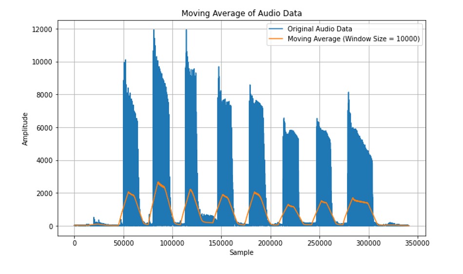
A moving average is a statistical technique used to analyse data by calculating averages of different subsets of the complete dataset, so if the moving average goes above a certain (normalized) threshold, we count it as a note, and when it falls back down, we deem that note as finished.

4. Putting it all together

We finally have all the tools to put everything together! Let’s use an example and go step by step, using the chart as a reference.

Here’s the bass file audio file we are going to use, it’s basically my friend playing a C Major scale, lets listen:

As we have mentioned in one of the previous chapters, we can dissect the binary data of the audio file to generate the geometric data as a sinusoidal wave below:

We then slice this bass file up using our moving averages algorithm, creating segments like the graph below:

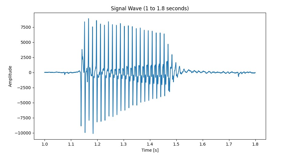
We then perform a Fourier transform to derive a fundamental frequency (human readable data), then cross reference the fundamental frequency to the note chart to find the final note!

The segment above derives us a C note, processing all the segments gives us this:

5. Summary

At its core, this project was about using C to read and interpret data in a meaningful way. However, what we learnt from this project goes beyond just learning a new language, it was really about pushing ourselves, delving out of the curriculum to learn more about a complex subject.

This was also an exercise in being comfortable with abstracting away certain concepts, as we couldn’t possibly learn everything there was to learn about audio and sound engineering, so we really had to be careful with which concepts we needed to understand fully (Fast Fourier Transforms etc) and what concepts we could just skim through.

This project also came with its fair share of obstacles, some of which were quite stressful to navigate given the timeline of this project during the school term. You can read about the full details of our technical challenges in our project report.

But looking back, it was fun embarking on this project, and it was definitely one of the more fulfilling ones in SUTD